ML 03 Classification
Algorithm Summary
-
k-NN is intuitive and simple but can be slow for large datasets.
-
Naive Bayes is fast and works well with high-dimensional data but assumes independent features.
-
Logistic Regression is a well-understood parametric approach, ideal for linearly separable data, and can handle regularization elegantly.
-
Decision Trees are highly interpretable but can overfit if not carefully regularized (via max depth, minimum samples per leaf, etc.).
| CATEGORY | CORE IDEA | MODEL TYPE | KEY HYPERPARAMETERS | STRENGTHS | WEAKNESSES | REGULARIZATION |
|---|---|---|---|---|---|---|
| k-NN | 1. Find k closest neighbors 2. Majority vote or average. |
Non-parametric | k: Number of neighbors. Distance metric |
Simple to implement. Minimal statistical assumptions. Models complex decision boundaries. |
Slow for large data. Bad in high-d space. Domain knowledge for good distance metric. |
Not typically applied, could use dimensionality reduction |
| Naive Bayes | Applies Bayes’ Theorem with a naive assumption of conditional independence among features | Probabilistic | Distribution choice (e.g. Multinomial) | Fast Robust with many features. Works well with small datasets. |
Bad if features are highly correlated. | Smoothing techniques to avoid zero probabilities. (e.g., Laplace smoothing) |
| Logistic Regression | Estimates the probability of each class via a linear combination of features passed through a sigmoid (or softmax) function, making it a parametric model. | Parametric | C: Inverse regularization strength. multi_class: One-vs-Rest or multinomial. Regularization type |
Interpretable coefficients. Can incorporate regularization Good when data is linearly (or log-linearly) separable. |
May struggle with highly non-linear relationships. Sensitive to outliers if regularization is not used properly. Assumes linear (or log-linear) deci-bound. |
L1 (Lasso) L2 (Ridge) Elastic Net: Combo of L1 and L2. |
| Decision Trees | Splits data into hierarchical branches based on feature values, aiming to maximize “purity” at each split. | Non-parametric | max_depth: Maximum tree depth. min_samples_leaf: Minimum samples required in a leaf node. Splitting criterion (e.g., Gini or Entropy). |
Highly interpretable Handles numeric & categorical Don't need scaling or dummies. Handles multi-output problems. |
Overfitting if grown without constraints. Greedy splitting may not yield a global optimum. Sensitive to data imbalance. Can struggle with certain complex interactions |
Indirectly via max_depth, min_samples_leaf, etc. Pruning can reduce overfitting |
Logistic
Sam
Target
-
Binary (Logit): Two classes (0 or 1).
-
Softmax Regression: Multiple classes (unordered); picks the class with the highest probability.
-
Ordered Logit: Multiple ordered classes.
\(probability(x) \: = \: \frac{1}{e^(-1 \: * \: regression \: model)}\)
Sam
Steps
-
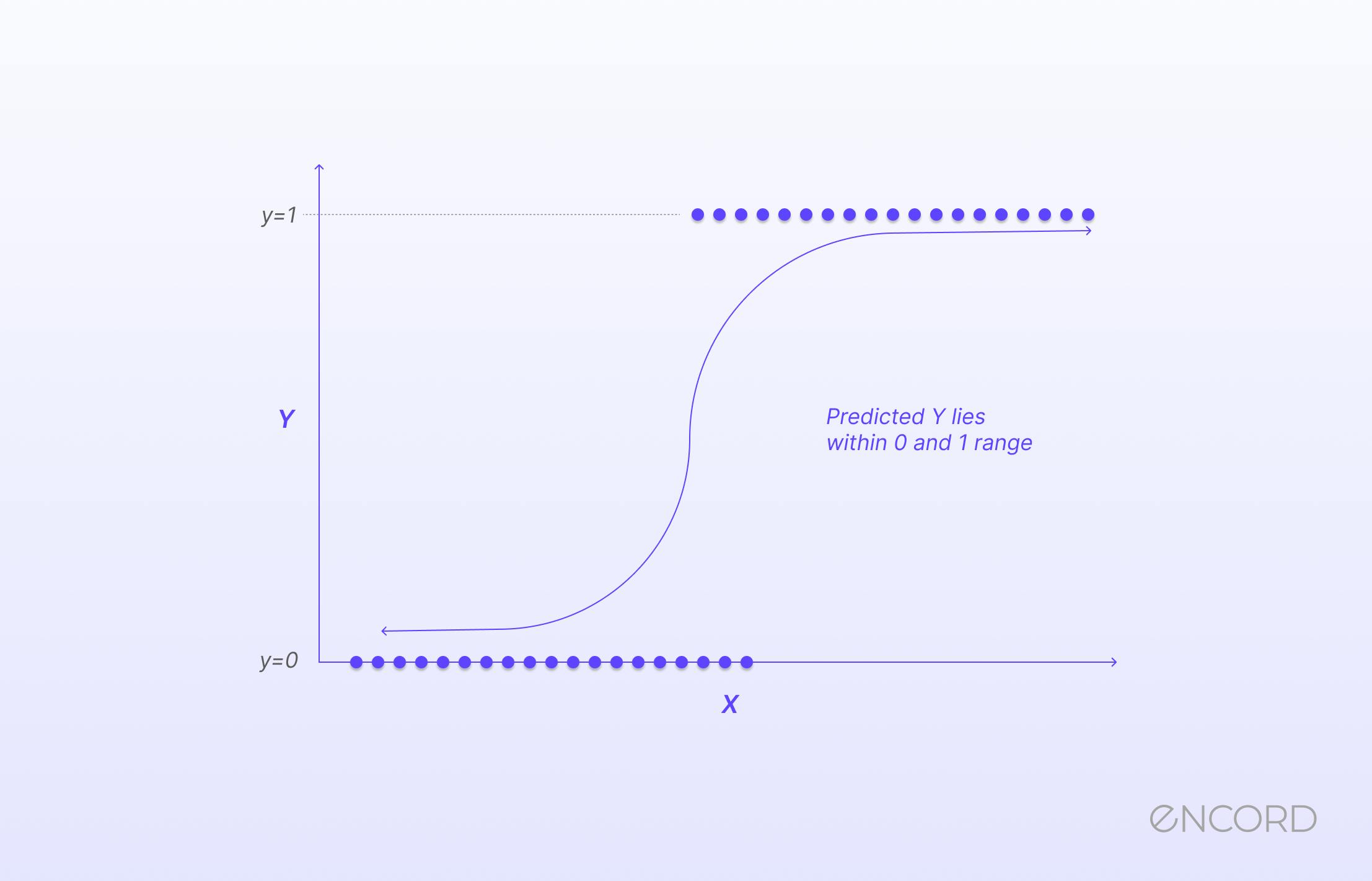
Compute linear score: Per observation, add up the weighted contribution of each variable (ie, model’s raw score).
-
Convert to probability: Pass that score through the S-shaped logistic curve to get a probability between 0 and 1.
-
Compare to reality: Check how far those probabilities are from the actual group labels (0/1).
-
Fit the model: Adjust the weights so the probabilities match reality as closely as possible across all observations.
-
Regularize (if needed): Add a penalty for overly large weights so the model stays simple and generalizes better.
-
Final model: Use the adjusted weights to make predictions on new data.
Regularization
Helps prevent overfitting by penalizing large coefficients.
| Type | Penalty | Key Characteristics |
|---|---|---|
| L1 (Lasso) | Sum of absolute values of weights | - Encourages sparsity (some coefficients may become zero) - Can be unstable with highly correlated features - Avoids using all features if many are redundant |
| L2 (Ridge) | Sum of squared values of weights | - Tends to shrink coefficients but rarely sets any to zero - More stable in the presence of correlated features |
| Elastic Net (L1 + L2) | Combination of L1 and L2 penalties | - Useful when multiple correlated features are suspected - Retains feature selection from L1 while benefiting from L2’s stability |
DT Purity
When deciding how to split a node, decision tree algorithms use measures like Gini Impurity or Entropy to assess how "pure" the resulting child nodes are.
| Measure | Range (Binary Setting) | Calculation | Characteristics |
|---|---|---|---|
| Gini Impurity | 0 (pure) to 0.5 (impure) | Uses squares of class probabilities | - Slightly faster to compute - Tends to isolate the most frequent class |
| Entropy | 0 (pure) to 0.5 (impure) | Uses logs of class probabilities | - Tends to produce more balanced splits |
Evaluation
Accuracy can be misleading. 2 primary reasons:
-
Imbalanced Class Distributions: When one class dominates, accuracy may inflate how well the model performs.
-
Ignoring Economic Costs/Benefits: Use a cost/benefit matrix to maximize profit.
Cost-Benefit Approach
-
Construct a “cost/benefit” matrix, detailing the financial impact of each type of prediction:
-
TP & TN: Represent revenue or benefits.
-
FP & FN: Represent costs or losses.
-
Multiply your confusion matrix by the cost/benefit matrix to calculate expected profit (or cost), and use this to guide decisions.
Formulas (TP, FP, TN, FN)
| Metric | Formula |
|---|---|
| True Positive Rate (TPR) / Recall | \(\frac{TP}{TP + FN}\) |
| False Positive Rate (FPR) | \(\frac{FP}{FP + TN}\) |
| Precision | \(\frac{TP}{TP + FP}\) |
| Recall (Same as TPR) | \(\frac{TP}{TP + FN}\) |
Model Evaluation Techniques
ChatGPT: Key "curves" and model evaluation techniques commonly used in classification:
Scope
-
Within: Evaluate a single model (diagnose overfitting, threshold tuning, and class imbalance)
-
Across: Compare multiple models, or compare model vs baseline.
-
Either
Scope |
Evaluation Technique | What | Why | Imbalanced Data Suitability |
|---|---|---|---|---|
| Within | Confusion Matrix | Shows counts of TP, TN, FP, FN | Derive performance metrics. | - |
| Within | ROC Curve Receiver Operating Characteristic |
Plots TPR vs. FPR at different probability thresholds. | Offers insight into the trade-off between TP & FP. | Bad. When negative class is large, the FPR remains deceptively low, which makes ROC curve look overly optimistic. |
| Either | AUC Area Under the ROC Curve |
A single-number summary (the area under the ROC curve). | \(\text{AUC} = 1\) indicates a perfect model. \(\text{AUC} = 0.5\) indicates a model with no discriminative power. |
- |
| Either | Precision-Recall Curve | Plots precision vs. recall as the decision threshold varies. | Especially useful for imbalanced datasets, or when false positives and false negatives incur high costs. | Good. Focuses on the minority class, where precision and recall are most critical. |
| Across | Lift Chart | Compares the model’s performance against a random baseline. | Shows how many more positives are identified by the model compared to random selection. | Good. Especially relevant if you’re trying to identify a small minority class more effectively than chance. |
| Across | Gain Chart | Displays cumulative gain (the fraction of positives identified) as you move through the sorted predictions. | Similar to Lift, it shows the improvement gained by the model over random selection. | Good. Like the Lift chart, it highlights model performance on minority classes. |
| Across | Cumulative Response Curve | Shows the proportion of positive instances captured as you move through the ranked predictions. | Commonly used in marketing and lead-generation applications to understand how quickly you capture most of the “yes” cases. | - |
| Within | Validation Curve | Plots the training and validation scores across different levels of model complexity (e.g., varying hyperparameters). | Helps diagnose overfitting or underfitting by showing whether the model performance is improving or plateauing. | - |
Single-Value Measures
| Metric | What | Why | Imbalanced Data Suitability |
|---|---|---|---|
| F-Measure (F1 Score) | The harmonic mean of precision and recall: \(F1 = 2 \times \frac{\text{Precision} \times \text{Recall}}{\text{Precision} + \text{Recall}}\) |
Combines precision and recall into a single metric, weighting them equally. | Good. Highlights performance on the minority class, where both precision and recall can be low. |
| Matthews Correlation Coefficient (MCC) | A correlation coefficient between observed and predicted classifications: \(\text{MCC} = \frac{(TP \times TN) - (FP \times FN)}{\sqrt{(TP + FP)(TP + FN)(TN + FP)(TN + FN)}}\) |
Accounts for all four quadrants (\(TP, TN, FP, FN\)) and provides a balanced measure even if the classes are of very different sizes. | Good. MCC is often more informative than accuracy and works well with imbalanced classes. |
| Cohen’s Kappa | Measures agreement between the model’s predictions and the true labels, adjusted for chance agreement. | In imbalanced scenarios, a model might appear good by randomly guessing the majority class. Kappa accounts for this chance agreement. | Mostly good. While it adjusts for chance, it can still be influenced by highly imbalanced distributions. |
Classification Code
Curves (Matrix, Precision/Recall, ROC)
# Knn
param_grid = dict(n_neighbors = list(range(1,31)),
weights = ["uniform", "distance"])
knn = KNeighborsClassifier()

# Tree
param_grid = dict(criterion = ["gini", "entropy"],
max_depth = range(2,10),
min_samples_leaf = range(2,8),
min_impurity_decrease = [0,1e-8,1e-7,1e-6,1e-5,1e-4])
grid_tree_clf = tree.DecisionTreeClassifier(random_state=45)

# Logistic
param_grid = dict(penalty = ['l1', 'l2'],
C = range(1,10))

# SVM
c = 5# reduce if overfitting
degrees = 3
influence = 1
poly_kernel_svm_clf = Pipeline([
 ("scaler", StandardScaler()),
 ("svm_clf", SVC(kernel="poly", degree=degrees, coef0=influence, C=c))
 ])
poly_kernel_svm_clf.fit(X, y)
# In text

from sklearn.metrics import classification_report
from sklearn import metrics

target_names = ['malignant', 'benign']
y_true = y_test
y_pred = y_pred

print(target_names)
print("Accuracy: {0:.2%}".format(accuracy_score(y_true, y_pred)))
print("Precision: {0:.2%}".format(metrics.precision_score(y_true, y_pred)))
print("Recall: {0:.2%}".format(metrics.recall_score(y_true, y_pred)))
print("F1: {0:.2%}".format(metrics.f1_score(y_true, y_pred)))
print('-------------------------------------')
print(classification_report(y_true, y_pred))
# Visually - https://i.imgur.com/PExd8UC.png

from sklearn.metrics import classification_report
from sklearn.metrics import confusion_matrix
print(classification_report(ytest, yfit, target_names=faces.target_names))

mat = confusion_matrix(ytest, yfit)
sns.heatmap(mat.T, square=True, annot=True, fmt='d', cbar=False,
xticklabels=faces.target_names,
yticklabels=faces.target_names)
plt.xlabel('true label')
plt.ylabel('predicted label');